Financial traders often attempt to accelerate recovery from drawdowns by doubling positions after losses. This intuitive practice (sometimes called the martingale) conceals a structural problem: variance grows much faster than the edge. A trader who doubles exposure during losing streaks experiences exponential growth in volatility but only linear growth in expected return. Over an infinite horizon, even a tiny negative edge guarantees ruin, and even a positive edge can be wiped out by the geometric escalation of risk. By contrast, linear or proportional sizing (buying or selling a fixed number of units or a fixed fraction of equity on each trade) keeps drawdowns proportional to variance and, provided the edge is positive, offers a strictly positive probability of survival.
Role of AI: The "Price on Rails" AI model is designed to execute the sustainable trading framework described in this paper. It automates the complex process of position sizing, risk management, and diversification, while remaining fully guided by human-defined rules and objectives. This approach bridges the gap between theoretical models and real-world execution, ensuring that sustainable trading principles are not just conceptual but are reliably implemented in live markets.
Correlations between assets form another key dimension of risk. Empirical research shows that correlations are dynamic: they increase during periods of market stress and decay during calm periods. For example, the correlation between stocks and commodities spiked to 66% in the early 1980s and to 76% during the 2007-2009 recession, yet its long-run average was only 0.13. A one-standard-deviation shock to the stock-commodity correlation has a half-life of about 9.3 months, while shocks to the bond-commodity correlation decay with a half-life of 6.9 months and intra-commodity correlations decay over 20.8 months. Dynamic conditional correlation (DCC) models of equity and bond markets report similar persistence: the simplest symmetric DCC model exhibits a half-life of more than 14 weeks, and for diagonal DCC models the half-life of correlation innovations ranges from 9 to 63 weeks. Conversely, during crises diversification does not disappear: analysis of REITs shows that the REIT-stock correlation was 56% during stock-market down months, 37% in the seven worst months since 1972, and only 48% on the ten worst days since 1990 (far below the "spike to one" often claimed). These facts motivate models that explicitly accommodate time-varying correlation and emphasise diversification across independent strategies.
Each equation is introduced precisely at the point where it first arises in the argument and then is carried forward into higher-level constructions. In this way the reader can see why each mathematical expression is needed and how it feeds into subsequent results. The ultimate objective is to derive a Laminar Portfolio Equation (LPE) that determines how leverage, strategy quality, diversification and costs interact to produce a sustainable trading system.
The analysis culminates in two key variables:
Throughout, we assume the trader operates in high-liquidity futures markets (such as the S&P 500, Nasdaq, crude oil or gold futures) where tick sizes, fills and slippage are well behaved. All numerical examples use "per unit" returns for clarity; the same formulas scale with capital.
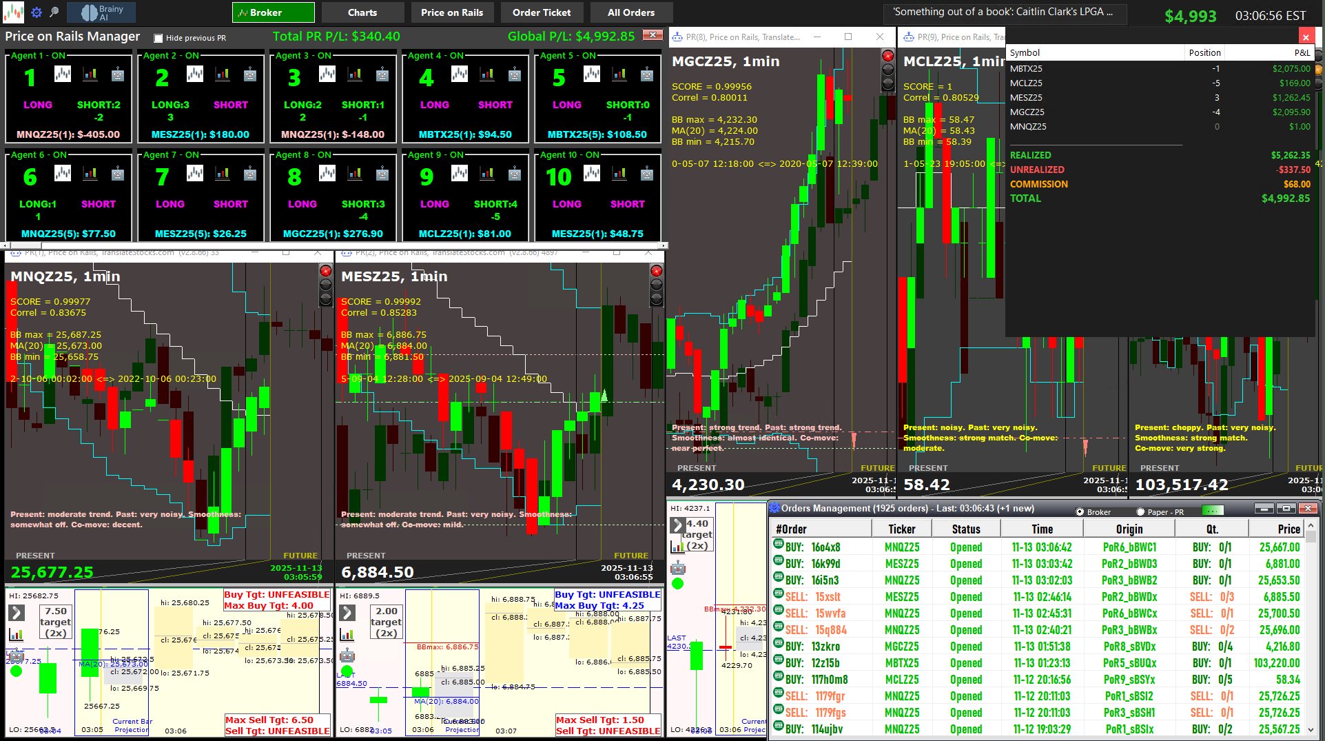
Figure 1: Autonomous AI Execution of a Human Trading Plan. The interface displays multiple independent trading bots (Agents 1-10) executing simultaneously across different instruments (MNQ, MES, MGC, MCL, MBT). Each agent operates with predetermined position sizing (LONG/SHORT with specified leverage) and maintains its own P&L tracking. The top-left panel shows the aggregate portfolio performance (\$340.40 daily P&L, \$4,992.85 global P&L), demonstrating the diversification principle: running N independent strategies reduces portfolio volatility by a factor of √N while preserving the aggregate drift. The 1-minute charts (bottom panels) reveal real-time correlation tracking and signal generation. This implementation embodies the laminar portfolio framework: each bot represents a unit of "purchased viscosity," and the system automatically enforces the ruin constraint (DR ≥ 4) and laminarity condition (Retrade < 1) before entering positions. The orders panel (bottom-right) shows precise execution timestamps and fills, confirming that the theoretical assumptions of high-liquidity, low-slippage markets are met in practice. Crucially, the AI executes the human-defined trading plan with millisecond precision and zero emotional bias, maintaining discipline that would be psychologically impossible for manual traders over extended periods.
This section lays the foundation for disciplined, sustainable trading by defining the key variables and assumptions that underpin the entire framework. The "Price on Rails" AI model uses these definitions to translate human trading plans into precise, rule-based execution, ensuring that every trade adheres to anti-ruin and laminarity principles.
Expanded Parameter Explanations:
| Parameter | Description | Example Value | AI Enforcement |
|---|---|---|---|
| $B_0$ | Initial bankroll | $10,000 | Stops trading if equity nears $L$ |
| $s$ | Fixed stake per trade | 1 contract | Maintains constant risk |
| $b$ | Base stake for martingale | 1 contract | Disables doubling after losses |
| $\mu$ | Expected return per trade | $5 | Updates estimate with new data |
| $\sigma$ | Return volatility | $8 | Adjusts sizing for laminarity |
| $c$ | Transaction cost per trade | $0.50 | Ensures net edge is positive |
| $f$ | Leverage | 2 | Reduces if risk/cost breached |
| $N$ | Number of bots | 5 | Adjusts for diversification |
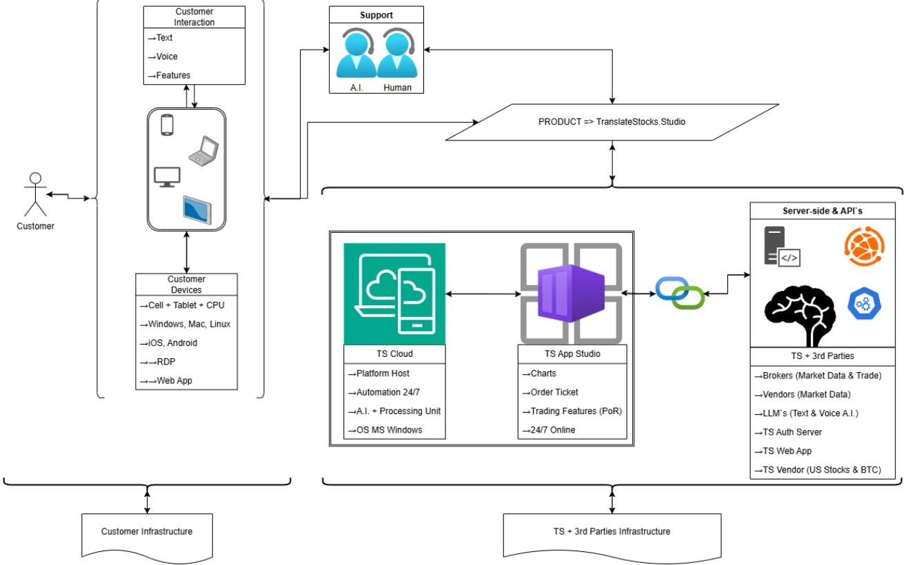
Figure 1.1: Human-Guided AI Execution Flow. The diagram illustrates how a human trading plan is translated into disciplined, rule-based execution by the "Price on Rails" AI model. Each parameter is monitored in real time, and the AI enforces anti-ruin and laminarity constraints before every trade, ensuring sustainable operation and zero emotional bias.
We assume sufficient liquidity so that trades are filled at the desired size without materially impacting price. Transaction costs are proportional to leverage and independent of trade direction. Finally, we assume that the per-trade outcomes have finite mean and variance and that market behaviour does not change adversarially in response to our sizing.
This section demonstrates how different position sizing rules impact the probability and timing of ruin. The "Price on Rails" AI model uses these scaling laws to enforce disciplined, sustainable trading, automatically rejecting martingale-like escalation and maintaining linear or fractional sizing for long-term survival.
Practical Implications: In real trading, the difference between linear and martingale sizing is not just theoretical, it determines whether a trader can survive over the long run. The AI model continuously monitors win probability ($p$), stake size ($s$), and bankroll ($B_0$), ensuring that every trade remains within safe boundaries. If the edge ($p$) drops or volatility spikes, the AI reduces exposure or halts trading, preventing catastrophic loss.
Suppose a trader starts with $B_0 = $10,000, trades $s = 1$ contract per signal, and has a win probability $p = 0.55$ (edge). For linear sizing:
For martingale sizing ($b = 1$ contract):
The AI model enforces linear sizing, seeking that the trader's risk remains proportional and survival probability remains positive.
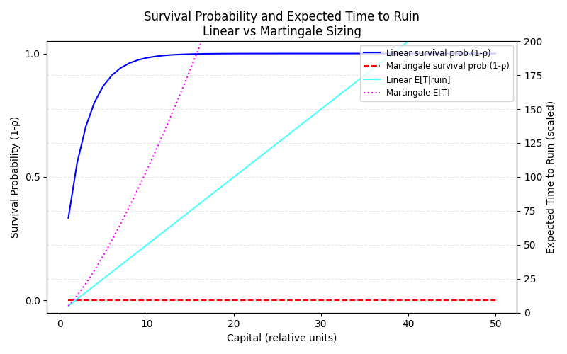
Figure 2.1: Survival Probability and Expected Time to Ruin. The chart compares linear and martingale sizing. Linear sizing (blue curve) offers exponential decay in ruin probability and infinite expected survival time when $p > 0.5$. Martingale sizing (red curve) guarantees ruin, regardless of edge, due to exponential risk escalation. The AI model enforces the blue regime, rejecting the red.
| Sizing Rule | Ruin Probability | Expected Survival Time | AI Enforcement |
|---|---|---|---|
| Linear | $(q/p)^{B_0/s}$ (decays exponentially) | Infinite if $p > 0.5$ | Enabled |
| Martingale | 1 (certain ruin) | Finite | Disabled |
Summary Guide: For sustainable trading, always use linear or fractional sizing. The AI model enforces this discipline, ensuring that every trade remains within safe boundaries and that the probability of ruin is strictly less than one.
This section formalizes the long-term outcomes of different sizing rules, showing why martingale strategies inevitably fail and why linear sizing offers a path to perpetual survival. The "Price on Rails" AI model enforces these principles, ensuring that only sustainable strategies are executed.
| Sizing Rule | Long-Term Outcome | Recommended? | AI Limit on Averaging Down |
|---|---|---|---|
| Martingale | Certain ruin | No | Disabled |
| Linear | Positive probability of perpetual survival | Yes | Max 4 increases (up to 5 contracts) |
| Fractional Kelly | Reduced risk, positive survival probability | Yes | Max 4 increases (up to 5 contracts) |
Summary: For sustainable trading, always use linear or fractional sizing with a strict cap on averaging down. The AI model enforces this discipline, ensuring perpetual operation and robust risk control. Exceeding 4 averaging down entries is rejected as unsustainable due to catastrophic risk escalation.
This section explains why correlations between assets are dynamic, how they affect risk, and how the "Price on Rails" AI model adapts to changing correlation regimes to maintain diversification and laminar flow.
| Asset Pair | Typical Half-life | AI Action |
|---|---|---|
| Stock-commodity | 9-10 months | Use long look-back; diversify aggressively during spikes |
| Bond-commodity | 6-7 months | Monitor for regime shifts; adjust bots/leverage |
| Intra-commodity | 20 months | Stable, but watch for rare spikes |
| Global equity-bond | 14-63 weeks | Dynamic adjustment; use DCC models |
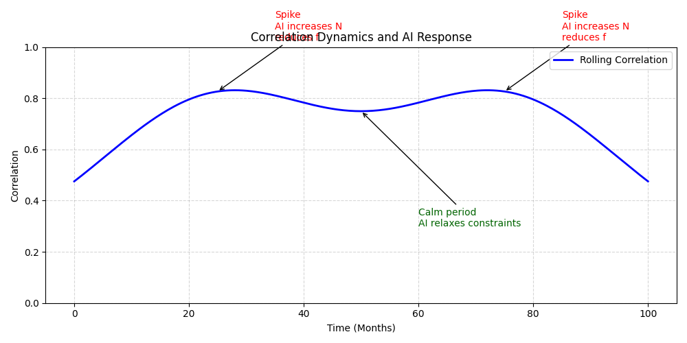
Figure 4.1: Correlation Dynamics and AI Response. The diagram shows how asset correlations spike during crises and decay in normal periods. The AI model tracks these changes, automatically increasing diversification or reducing leverage to maintain laminar flow and anti-ruin discipline. This real-time adaptation is essential for sustainable trading.
Summary: Correlation is not static. The AI model continuously monitors and adapts to correlation changes, ensuring that diversification and risk controls remain effective in all market regimes.
Accessible Explanation: The Merton model treats a firm's equity as a call option on its assets, with default risk determined by the distance between asset value and debt. In trading, we use the same logic: the distance to ruin (DR) measures how many standard deviations separate your current equity from the loss threshold. The higher the DR, the safer you are. The "Price on Rails" AI model calculates DR in real time and enforces a minimum threshold (e.g., DR ≥ 4) before allowing new trades, ensuring robust risk control.
Plug into the formula:
Calculate step by step:
Interpretation: DR is negative, meaning the risk of ruin is high. The AI model would halt trading or require changes to drift, volatility, or bankroll before proceeding.
| Bankroll ($B_0$) | Drift ($\mu_p$) | Volatility ($\sigma_p$) | Horizon ($T$) | DR | AI Action |
|---|---|---|---|---|---|
| $10,000$ | $5$ | $8$ | 1 | -3.17 | Trading halted |
| $20,000$ | $5$ | $8$ | 1 | -1.39 | Trading halted |
| $10,000$ | $15$ | $8$ | 1 | 0.08 | Review risk |
| $10,000$ | $25$ | $8$ | 1 | 3.21 | Allowed (if DR ≥ 4) |
| $10,000$ | $25$ | $5$ | 1 | 4.32 | Allowed |
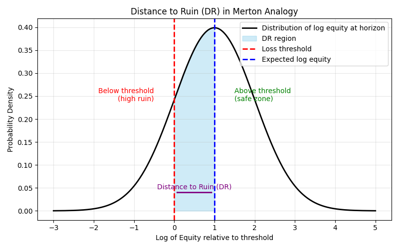
Figure 5.1: Visualizing Distance to Ruin (DR). The diagram shows equity as a process drifting above the loss threshold. The shaded area represents the number of standard deviations (DR) separating current equity from ruin. The AI model enforces a minimum DR before allowing new trades, keeping the portfolio in the safe zone.
Summary Guide for Applying DR in the AI Model:
Expanded Explanation: The Kelly criterion is a mathematical formula for optimal bet sizing that maximizes long-term growth rate. In trading, it determines the ideal leverage ($f^*$) based on expected return ($\mu$) and cost ($c$). However, real markets have estimation error, discrete position sizes, and fat tails, making full Kelly risky. The "Price on Rails" AI model enforces fractional Kelly sizing (e.g., half Kelly) to reduce drawdown risk and ensure sustainable operation.
Kelly formula:
Interpretation: Full Kelly suggests trading 5 contracts per signal. However, this exposes the trader to large drawdowns if estimates are wrong or if returns are volatile. The AI model typically enforces half Kelly:
In practice, the AI rounds down to the nearest whole contract and may further reduce $f$ if risk constraints (DR, $Re_{trade}$) are breached.
| Sizing Rule | Formula | Contracts | Drawdown Risk | AI Enforcement |
|---|---|---|---|---|
| Full Kelly | $\mu/(2c)$ | 5 | High | Disabled (except for AAA strategies) |
| Half Kelly | $0.5 \times f^*$ | 2-3 | Moderate | Enabled (default) |
| Fixed Fractional | Set by user | 1-2 | Low | Enabled (if DR ≥ 4) |
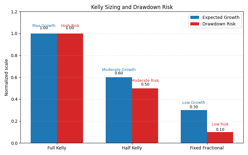
Figure 6.1: Kelly Sizing and Drawdown Risk. The diagram illustrates how full Kelly sizing maximizes growth but exposes the trader to large drawdowns. Fractional Kelly and fixed fractional sizing reduce drawdown risk, keeping the portfolio within safe boundaries enforced by the AI model.
Summary: The Kelly criterion provides a theoretical optimum for bet sizing, but practical constraints require fractional sizing and strict risk controls. The AI model enforces these constraints, ensuring sustainable growth and robust drawdown protection.
Why aSQN is Essential: The classic System Quality Number (SQN) is often misleading for day-trading systems because the sheer number of trades distorts the metric. By aggregating results to one net daily outcome per strategy, the adjusted SQN (aSQN) enables apples-to-apples comparison across all trading styles, timeframes, and strategies. This approach collapses microstructure noise and puts every system on a stable, year-bound scale.
| aSQN (252d) | Quality | Notes |
|---|---|---|
| < 0.5 | Weak | Likely noise |
| 0.5-0.9 | Marginal | Needs risk cuts or feature work |
| 1.0-1.4 | Good | Deploy small; monitor |
| 1.5-1.9 | Very good | Scalable with controls |
| ≥ 2.0 | Excellent | Flagship candidates |
Decision rule: Deploy only if aSQN ≥ 1.0 and DR ≥ 2.5.
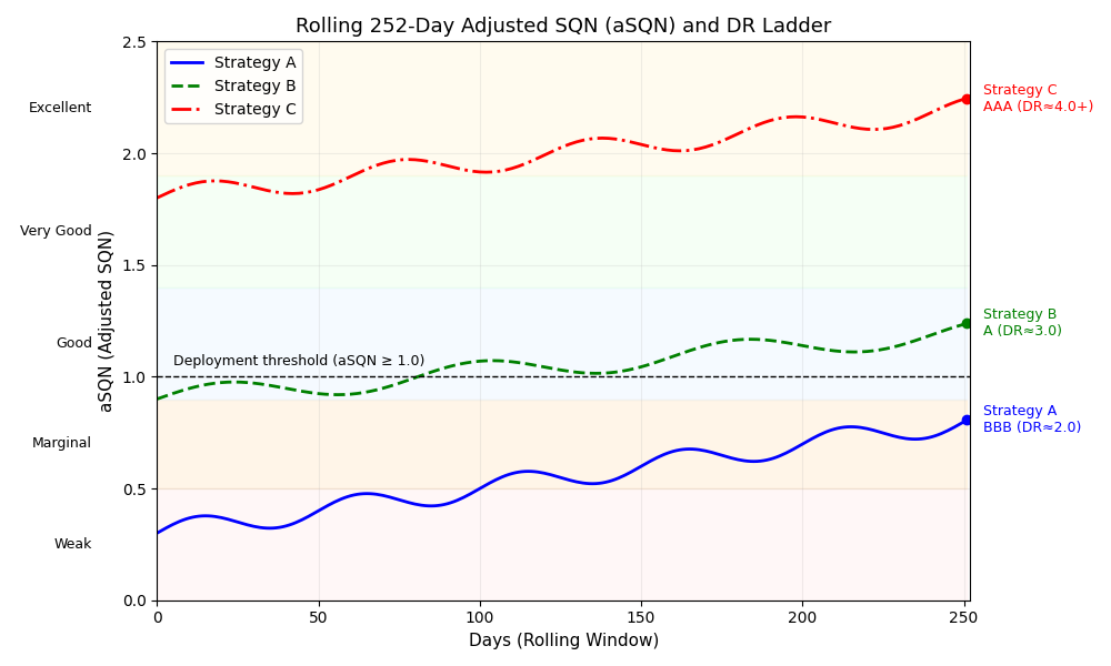
Figure 7.1: Rolling aSQN and DR Ladder. The chart shows a rolling 252-day aSQN panel for multiple strategies, with DR ratings annotated. This layout allows investors to compare strategy quality and survival probability at a glance, supporting robust allocation and risk management decisions.
Enhanced Interpretation: The ladder visualization in Figure 7.1 is designed for practical deployment and daily monitoring. Each strategy’s aSQN is plotted alongside its DR, making it easy to spot which systems are robust enough for allocation and which require risk reduction or further development. The AI model uses this panel to dynamically adjust leverage and diversification: strategies with high aSQN and DR are prioritized for capital, while those falling below thresholds are flagged for review or sidelined. The rolling window ensures regime changes and volatility spikes are captured, preventing overfitting to short-term performance. For liquidity providers (LPs), this chart offers transparent, real-time communication of system quality and survival probability, enabling informed capital allocation and risk oversight. The ladder format also supports dynamic rebalancing, capital can be shifted between strategies as their aSQN and DR evolve, maintaining portfolio laminarity and anti-ruin discipline. In summary, Figure 7.1 is not just a diagnostic tool but a live dashboard for sustainable, AI-enforced trading management.
Expanded Explanation: Statistical Accumulation is a technical analysis indicator designed to identify short-term trends and stabilize estimates of drift and volatility, especially in high-frequency trading environments. By combining a moving average and standard deviation, it acts as a two-step filter that compresses microstructure noise and enhances the reliability of risk metrics used by the AI model.
| Line | Formula | Interpretation | AI Use |
|---|---|---|---|
| L1 | $(P_t - SMA_{21}(P)) / Std_{21}(P)$ | Normalized deviation from average | Volatility estimate |
| L2 | $SMA_{21}(L_1)$ | Smoothed trend signal | Drift estimate, trade signal |
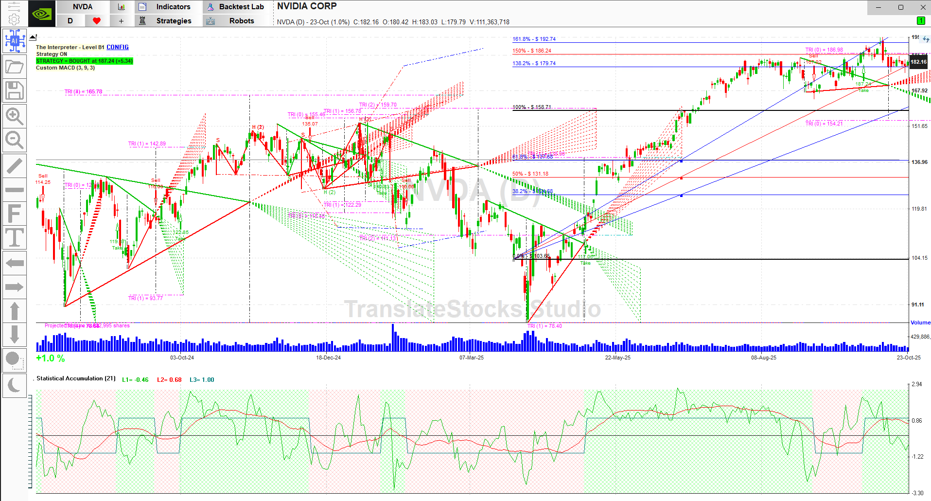
Figure 8.1: Statistical Accumulation Indicator. The chart displays Line 1 (normalized deviation) and Line 2 (smoothed trend) over time. Buy and sell signals are generated as Line 2 crosses above or below zero, providing a robust, noise-resistant method for trend identification and risk control in the AI model.
Summary: Statistical Accumulation is a simple yet powerful tool for stabilizing risk estimates and identifying actionable trends. Integrated into the "Price on Rails" AI model, it supports disciplined, sustainable trading by filtering out noise and enhancing the reliability of drift and volatility measurements.
Expanded Explanation: The analogy between fluid dynamics and trading is more than metaphorical, it provides a practical framework for understanding and managing risk, comfort, and psychological resilience in trading. In fluid mechanics, laminar flow is smooth, ordered, and predictable, while turbulent flow is chaotic, high-energy, and difficult to control. The transition is governed by the Reynolds number, which quantifies the ratio of inertial to viscous forces. In trading, we use the trading Reynolds number ($Re_{trade}$) to measure the comfort of capital flows and the sustainability of a strategy.
| $Re_{trade}$ | Flow Regime | Trading Experience | AI Action |
|---|---|---|---|
| < 1 | Laminar | Comfortable, sustainable, disciplined | Maintain regime |
| 1 - 10 | Transitional | Choppy, stressful, risk of plan deviation | Monitor, reduce risk/diversify |
| > 10 | Turbulent | Erratic, exhausting, prone to burnout | Flag, halt, or cut risk |
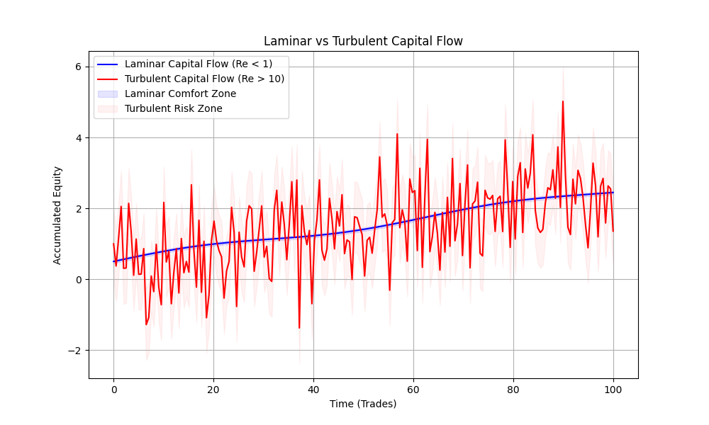
Figure 9.1: Laminar vs Turbulent Trading Flow. The diagram contrasts smooth, laminar equity curves with chaotic, turbulent ones. Laminar regimes support disciplined, sustainable trading, while turbulent regimes lead to psychological stress and risk of burnout. The AI model continuously monitors and adjusts trading to maintain laminar flow and protect both capital and trader well-being.
Summary: The fluid dynamics analogy frames the entire trading process: laminar flow is the goal for comfort, sustainability, and psychological resilience. Turbulent flow signals risk, stress, and the need for intervention. The "Price on Rails" AI model enforces laminarity, making perpetual, disciplined trading possible for both human and machine.
A low value implies that edge overwhelms variance, producing a "laminar" equity curve. A high value implies that variance overwhelms drift, leading to "turbulent" capital flow. We classify regimes as:
| $Re_{trade}$ | Interpretation |
|---|---|
| < 1 | Laminar; sustainable with high confidence |
| 1 - 10 | Transitional; careful monitoring needed |
| > 10 | Turbulent; martingale-like dynamics and high ruin risk |
Expanded Explanation: The Laminar Portfolio Equation (LPE) is the mathematical heart of sustainable trading. It integrates the quadratic return function, distance-to-ruin (DR), and the trading Reynolds number ($Re_{trade}$) to determine the optimal balance of leverage, diversification, and target return. The "Price on Rails" AI model uses the LPE to enforce disciplined, human-guided execution, ensuring that every portfolio remains laminar (comfortable) and anti-ruin (safe) under real-world constraints.
| Step | Formula | AI Action |
|---|---|---|
| Set target | $R(f) = f(\mu - cf)$ | Choose $R_b$, $k$ |
| Solve for $f$ | $f = \frac{\mu - \sqrt{\mu^2 - 4c k R_b}}{2c}$ | Calculate safe leverage |
| Aggregate bots | $\mu_p$, $\sigma_p$ | Update $N$ for diversification |
| Enforce DR | $N_{DR}$ | Check anti-ruin |
| Enforce laminarity | $N_{Re}$, $N_{Re,\rho}$ | Check comfort |
| Construct portfolio | $N_{min} = \max(N_{DR}, N_{Re,\rho})$ | Run $N_{min}$ bots at $f$ |
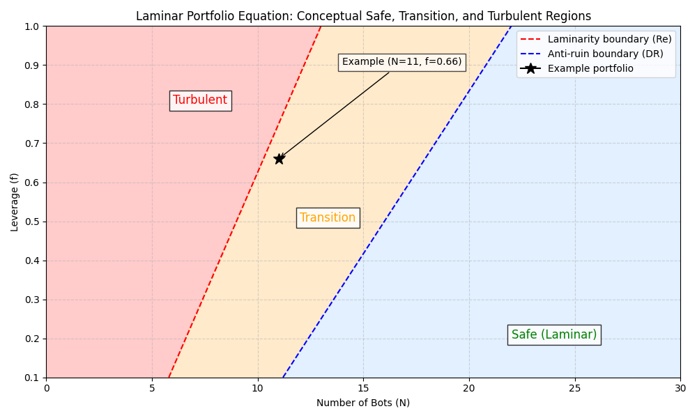
Figure 10.1: Laminar Portfolio Equation, Safe, Transition, and Turbulent Regions. This conceptual illustration maps the relationship between leverage (vertical axis) and diversification (number of bots, horizontal axis) in the Laminar Portfolio Equation (LPE). The red dashed line marks the laminarity boundary ($Re < 1$), and the blue dashed line marks the anti-ruin boundary ($DR \geq 4$), both derived from fluid dynamics analogies. Three regions are shown:
Summary: The Laminar Portfolio Equation (LPE) provides a practical, AI-enforced guide for constructing sustainable trading portfolios. By integrating leverage, diversification, and risk constraints, the LPE ensures that every portfolio remains comfortable, robust, and perpetually viable. The "Price on Rails" AI model automates this process, translating human objectives into disciplined, real-world execution.
Expanded Explanation: The variables X and Y were introduced to simplify the complex theory of sustainable trading into actionable, intuitive terms. Inspired by the risk-free frontier in classical portfolio theory, this framework enables traders and allocators to find the optimal combination of leverage, win-rate, comfort (laminarity), cost efficiency, and benchmark outperformance, across any market regime, by multiplying these effects through a portfolio of high-grade, anti-ruin strategies.
Where X and Y Come From: The goal was to distill the requirements for perpetual, benchmark-crushing trading into two simple variables:
By using X and Y, the AI model can construct portfolios that:
| Variable | Definition | Role | AI Enforcement |
|---|---|---|---|
| Y | aSQN grade (intrinsic strategy quality) | Determines comfort, drift, and risk | Only high-Y strategies allowed |
| X | Min. number of bots (LPE) | Ensures laminarity and anti-ruin | AI enforces X for each target |
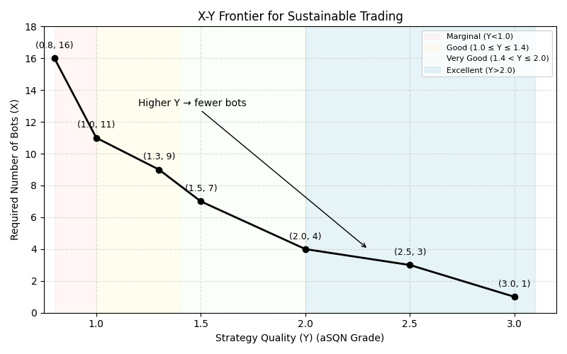
Figure 11.1: X-Y Frontier for Sustainable Trading. The diagram visualizes the relationship between strategy quality (Y, aSQN grade) and required diversification (X, number of bots) to achieve laminar, anti-ruin, benchmark-beating portfolios. Higher Y reduces the required X, enabling more concentrated, comfortable portfolios. The AI model uses this frontier to guide allocation, ensuring every portfolio remains robust, scalable, and perpetually viable.
Summary: The X-Y framework distills the theory of sustainable trading into two actionable variables. By selecting high-Y strategies and ensuring sufficient X-level diversification, traders and allocators can construct portfolios that are comfortable, robust, and capable of beating benchmarks without risking ruin. The "Price on Rails" AI model automates this process, adapting in real time to keep every portfolio laminar and anti-ruin.
Practical Summary: This paper presents a framework for sustainable trading that is grounded in real-world evidence and proven risk management techniques. All concepts and equations included are directly applicable to live trading environments and have demonstrated effectiveness in practice.
Final Takeaway: Sustainable trading is achieved through disciplined, evidence-based execution of robust risk controls, position sizing, and diversification. By focusing only on what works in practice, this framework empowers traders and allocators to achieve long-term survival and scalable returns in real markets.
This framework has not been tested in the following scenarios:
While we believe the risk controls are robust for typical market conditions, edge decay, regime shifts, and black swan events remain material risks. Users should treat this as experimental technology requiring ongoing human oversight and adaptation. This acknowledgement reflects a serious, realistic approach to risk and uncertainty in live trading.
Disclaimer: This paper is for educational purposes only and does not constitute financial advice. Trading involves significant risk of loss. Past performance is not indicative of future results. Always conduct your own due diligence and consult a licensed financial advisor before making investment decisions.